41 excel column chart labels
peltiertech.com › excel-column-Column Chart with Primary and Secondary Axes - Peltier Tech Oct 28, 2013 · Plot data in clustered column chart (Chart 1). Assign Sec 1 & Sec 2 to secondary axis (Chart 2). Set primary Y axis scale to 0 min and 6 max, set secondary Y axis scale to -30 min and +30 max (Chart 3). Use custom number format [<=3]0;;; for primary axis tick labels, use custom number format 0;;0; for secondary axis tick labels (Chart 4). How to Directly Label Stacked Column Charts in Excel - simplexCT On the worksheet, right-click the chart and then, on the shortcut menu, click Select Data. 4. Next, In the Select Data Source dialog box, click on the Add button under Legend Entries (Series). 5. In the Edit Series dialog box, type "Labels" in the Series name edit box and refer to cell B13 in the Series values edit box as per the below screenshot:
Change the format of data labels in a chart To get there, after adding your data labels, select the data label to format, and then click Chart Elements > Data Labels > More Options. To go to the appropriate area, click one of the four icons ( Fill & Line, Effects, Size & Properties ( Layout & Properties in Outlook or Word), or Label Options) shown here.
Excel column chart labels
How to Make a Column Chart in Excel: A Guide to Doing it Right In this chart, each column is the same height making it easier to see the contributions. Using the same range of cells, click Insert > Insert Column or Bar Chart and then 100% Stacked Column. The inserted chart is shown below. A 100% stacked column chart is like having multiple pie charts in a single chart. Multiple Series in One Excel Chart - Peltier Tech Aug 09, 2016 · The X labels specified in the first series formula is what Excel uses for the chart. If we had selected only the new Y values, ignoring any new X values, and kept Categories in First Column unchecked, both series formulas would reference the same X label range. Data Labels in Excel Pivot Chart (Detailed Analysis) 7 Suitable Examples with Data Labels in Excel Pivot Chart Considering All Factors 1. Adding Data Labels in Pivot Chart 2. Set Cell Values as Data Labels 3. Showing Percentages as Data Labels 4. Changing Appearance of Pivot Chart Labels 5. Changing Background of Data Labels 6. Dynamic Pivot Chart Data Labels with Slicers 7.
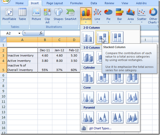
Excel column chart labels. Text Labels on a Horizontal Bar Chart in Excel - Peltier Tech Dec 21, 2010 · In Excel 2003 the chart has a Ratings labels at the top of the chart, because it has secondary horizontal axis. Excel 2007 has no Ratings labels or secondary horizontal axis, so we have to add the axis by hand. On the Excel 2007 Chart Tools > Layout tab, click Axes, then Secondary Horizontal Axis, then Show Left to Right Axis. › excel-stacked-column-chartStacked Column Chart in Excel (examples) - EDUCBA This has been a guide to Stacked Column Chart in Excel. Here we discuss its uses and how to create Stacked Column Chart in Excel with excel examples and downloadable excel templates. You may also look at these useful functions in excel – Interactive Chart in Excel; Freeze Columns in Excel; Excel Clustered Column Chart; Excel Column Chart How to show percentages in stacked column chart in Excel? - ExtendOffice Add percentages in stacked column chart. 1. Select data range you need and click Insert > Column > Stacked Column.See screenshot: 2. Click at the column and then click Design > Switch Row/Column.. 3. In Excel 2007, click Layout > Data Labels > Center.. In Excel 2013 or the new version, click Design > Add Chart Element > Data Labels > Center.. 4. How-to Add Centered Labels Above an Excel Clustered Stacked Column Chart Step-by-Step tutorial is available at: I posted how you can easily create a clustered stacked column chart in...
Stacked Column Chart in Excel (examples) - EDUCBA Here we discuss how to create Stacked Column Chart in Excel with excel examples and downloadable excel templates. EDUCBA. MENU MENU. Free Tutorials; Certification Courses; 120+ Courses All in One Bundle; ... Overlapping of data labels, in some cases, this is seen that the data labels overlap each other, and this will make the data to be ... peltiertech.com › multiple-series-in-one-excel-chartMultiple Series in One Excel Chart - Peltier Tech Aug 09, 2016 · The X labels specified in the first series formula is what Excel uses for the chart. If we had selected only the new Y values, ignoring any new X values, and kept Categories in First Column unchecked, both series formulas would reference the same X label range. How to add data labels from different column in an Excel chart? This method will guide you to manually add a data label from a cell of different column at a time in an Excel chart. 1.Right click the data series in the chart, and select Add Data Labels > Add Data Labels from the context menu to add data labels.. 2. › documents › excelHow to add total labels to stacked column chart in Excel? Select the source data, and click Insert > Insert Column or Bar Chart > Stacked Column. 2. Select the stacked column chart, and click Kutools > Charts > Chart Tools > Add Sum Labels to Chart. Then all total labels are added to every data point in the stacked column chart immediately. Create a stacked column chart with total labels in Excel
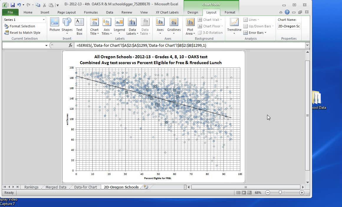
Line Column Combo Chart Excel | Line Column Chart | Two Axes Creating a Line Column Combination Chart in Excel . You can create a combination chart in Excel but its cumbersome and takes several steps. Select your data and then click on the Insert Tab, Column Chart, 2-D Column. Note: Make sure your labels are formatted as text or they will be added to the chart as a third set of bars. Next, right click on ... How to Add Labels to Scatterplot Points in Excel - Statology Step 3: Add Labels to Points. Next, click anywhere on the chart until a green plus (+) sign appears in the top right corner. Then click Data Labels, then click More Options…. In the Format Data Labels window that appears on the right of the screen, uncheck the box next to Y Value and check the box next to Value From Cells. Adding Labels to Column Charts | Online Excel Training | Kubicle To add data labels, just right-click on a data series and click add data labels. To see the data labels clearly, I'll need to select them and change their color to white. The data labels are determined by the vertical axis of your chart. Currently, the vertical axis shows millions, therefore, my data labels are shown in millions as well. Column Chart with Category Axis Labels Between Columns Select the added series by selecting the green bars and clicking the up arrow key. Click the menu key (between the right Alt and Ctrl buttons on most Windows keyboards) or hold Shift and click the F10 function key to pop up the context menu. Click Change Series Chart Type, and choose XY Scatter. This adds a set of markers along the bottom of ...
X-Y Chart (Excel 2010) - Step 2 Construct a Scatter Chart with Labels - YouTube
› documents › excelHow to add data labels from different column in an Excel chart? How to add total labels to stacked column chart in Excel? For stacked bar charts, you can add data labels to the individual components of the stacked bar chart easily. But this article will introduce solutions to add a floating total values displayed at the top of a stacked bar graph so that make the chart more understandable and readable.
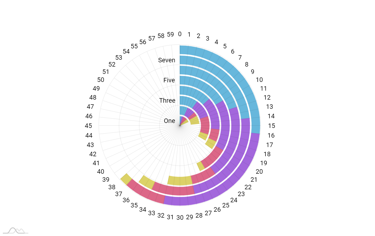
Radial bar chart - amCharts
Excel Custom Chart Labels • My Online Training Hub Note: Excel 2013 onward also requires this step if you have more than one series you want to position your labels above. Step 1: Select cells A26:D38 and insert a column Chart. Step 2: Select the Max series and plot it on the Secondary Axis: double click the Max series > Format Data Series > Secondary Axis: Step 3: Insert labels on the Max ...

Microsoft Excel Charts – Office Tutorial
Column Chart in Excel | How to Make a Column Chart? (Examples) Clustered Column Chart: A clustered chart in Excel presents more than one data series in clustered vertical columns. Each data series shares the same axis labels, so vertical bars are grouped by category. The clustered columns can make the direct comparison of multiple series and can show change over time.

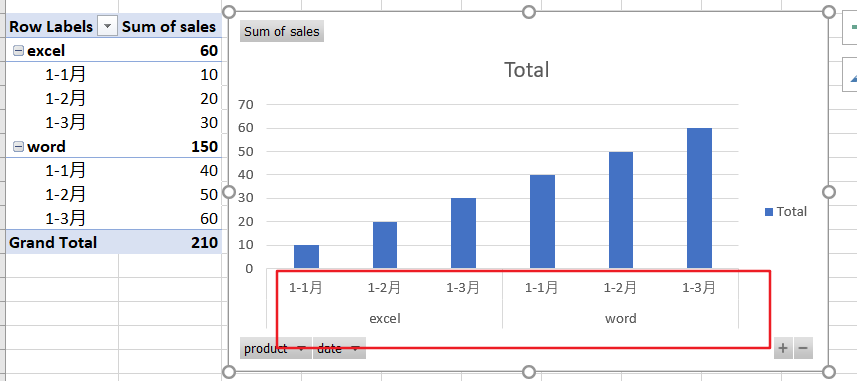
How to Create Multi-Category Chart in Excel - Excel Board
How to Add Labels to Show Totals in Stacked Column Charts in Excel The chart should look like this: 8. In the chart, right-click the "Total" series and then, on the shortcut menu, select Add Data Labels. 9. Next, select the labels and then, in the Format Data Labels pane, under Label Options, set the Label Position to Above. 10. While the labels are still selected set their font to Bold. 11.
29 Label Columns In Excel - 1000+ Labels Ideas
How to group (two-level) axis labels in a chart in Excel? - ExtendOffice (1) In Excel 2007 and 2010, clicking the PivotTable > PivotChart in the Tables group on the Insert Tab; (2) In Excel 2013, clicking the Pivot Chart > Pivot Chart in the Charts group on the Insert tab. 2. In the opening dialog box, check the Existing worksheet option, and then select a cell in current worksheet, and click the OK button. 3.
Printable 3 Column Spreadsheet Printable Spreadshee printable 3 column spreadsheet.
Add or remove data labels in a chart - support.microsoft.com Click the data series or chart. To label one data point, after clicking the series, click that data point. In the upper right corner, next to the chart, click Add Chart Element > Data Labels. To change the location, click the arrow, and choose an option. If you want to show your data label inside a text bubble shape, click Data Callout.

31 How To Label Excel Columns - Labels Database 2020
Change axis labels in a chart - support.microsoft.com Right-click the category labels you want to change, and click Select Data. In the Horizontal (Category) Axis Labels box, click Edit. In the Axis label range box, enter the labels you want to use, separated by commas. For example, type Quarter 1,Quarter 2,Quarter 3,Quarter 4. Change the format of text and numbers in labels
Excel Dashboard Templates How-to Put Percentage Labels on Top of a Stacked Column Chart - Excel ...
Edit titles or data labels in a chart - support.microsoft.com On a chart, click the label that you want to link to a corresponding worksheet cell. On the worksheet, click in the formula bar, and then type an equal sign (=). Select the worksheet cell that contains the data or text that you want to display in your chart. You can also type the reference to the worksheet cell in the formula bar.
Post a Comment for "41 excel column chart labels"